The zip file dtcwpt.zip contains MATLAB programs and filters that implement the DT-CWPT. The explanation below uses fragments of code from the file "demo.m".
The dual-tree complex wavelet packet transform involves two DWPT's (discrete wavelet packet transform). The MATLAB functions 'DTCWPT.m' and 'IDCWPT.m' implement the forward and inverse transforms for a single DWPT. The forward transform 'DTCWPT.m' requires three PR filter sets, namely (referring to Figure-6 in the paper) the first stage filters (H1(1)), Hi (Hi' for the second DWPT) and Fi (for both DWPTs). Also, the number of levels must be specified. First, let's load the filters :
>> load dtcwpt_filters;
>> who
Your variables are:
f first_1 first_2 g h
Each variable above is a 2-row matrix where the first row contains the lowpass filter and the second row the highpass filter.
'h' corresponds to Hi (referring to the paragraph above);
'g' to Hi';
'f' to Fi;
and 'first_1' and 'first_2' are the first stage filters for the first and the second DWPT. The filters in 'first_1' and 'first_2' are related by a unit shift.
>> first_1
first_1 =
0.1601 0.6038 0.7243 0.1384 -0.2423 -0.0322 0.0776 -0.0062 -0.0126 0.0033
0.0033 0.0126 -0.0062 -0.0776 -0.0322 0.2423 0.1384 -0.7243 0.6038 -0.1601
>> first_2
first_2 =
0 0.1601 0.6038 0.7243 0.1384 -0.2423 -0.0322 0.0776 -0.0062 -0.0126 0.0033
0 0.0033 0.0126 -0.0062 -0.0776 -0.0322 0.2423 0.1384 -0.7243 0.6038 -0.1601
In these sets of filters only 'h' and 'g' are special in that they approximately satisfy a certain property (half-shift) sufficient to implement the dual-tree complex wavelet transform. Here, the filters are Kingsbury's Q-shift filters. The remaining sets of filters can be arbitrary PR filters (orthogonality is not necessary). These filters in 'dtcwpt_filters.mat' are set to be Daubechies filters with 5 and 6 vanishing moments.
To demonstrate the usage of the functions, let's check perfect reconstruction by defining a random signal and performing the forward and inverse transforms with 3 levels using the loaded filters.
>> x = rand(1,512);
>> y = DTWPT(x,first_1,h,f,3);
The output is a cell array where each cell holds a particular subband. Continuing,
>> xx = IDTWPT(y,first_1(:,end:-1:1),h(:,end:-1:1),f(:,end:-1:1));
>> max(abs(x-xx))
ans =
3.9635e-014
verifying perfect reconstruction.
The 'defining property' for the DTCWPT is that the underlying discrete basis functions in the two DWPTs are discrete Hilbert transform pairs. We can verify that this property is approximately satisfied by picking two elements from the discrete bases using the the inverse transform. For this, we transform the zero signal and in the transform domain, set the same coefficient in each DWPT to 1. The results of the inverse transforms should approximately be a discrete Hilbert transform
pair. We use a 4-level DWPT below.
>> x = zeros(1,1024);
>> y = DTWPT(x,first_1,h,f,4);
>> y{7}(30) = 1;
>> x1 = IDTWPT(y,first_1(:,end:-1:1),h(:,end:-1:1),f(:,end:-1:1));
>> x2 = IDTWPT(y,first_2(:,end:-1:1),g(:,end:-1:1),f(:,end:-1:1));
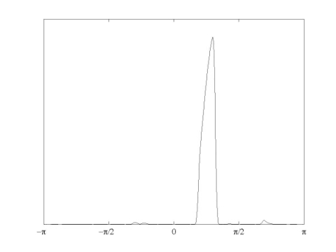
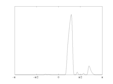
The Hilbert transform relationship among the sequences 'x1' and 'x2' can be verified by looking at the DFT of the signal 'x1-i*x2'.
The figure verifies our expectation. Notice however that there's a disturbingly significant bump. This is a shortcoming of discrete wavelet packet transforms, when the filters are far from being ideal half-band rectangular frequency response filters. One modification then is to use longer filters approximating this ideal behavior. Actually, replacing the first stage filters and 'f' in 'dtcwpt_filters.mat', we obtain a more desired behavior, as shown below (an improvement in all of the subbands can be observed but still some subbands have these undesired secondary bumps). The filters used are from 'dtcwpt_filters_longer.mat'.