Expectation-Maximization Algorithm

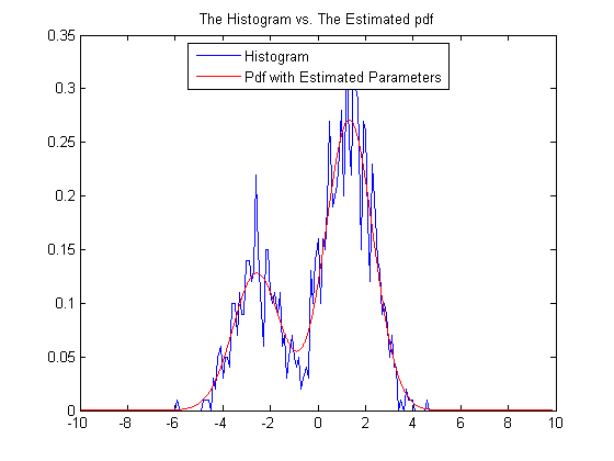
We assume that the data consists of a Gaussian mixture with two components with unit variance. The weights and the means of the components are unknown. We demonstrate their estimation via the EM algorithm as discussed in class.

% the unknown parameters
alp = rand(1,1); % this is the probability that z = 1
th = randn(2,1)*3; % the unknowm means

% produce the data
n = 1000; % number of observations.

z = double( rand(n,1) < alp ); % hidden states
x = randn(n,1) + th(1).*(1-z) + th(2).*z; % observations


% initialization
Ealp = 1/2;
Eth = [0; 1];

% gaussian pdf
g = @(x,m) (1/sqrt(2*pi))*exp(-0.5*(x-m).^2);

% mixture pdf
f = @(x,m,bet) (1-bet) * (1/sqrt(2*pi)) * exp(-0.5*(x-m(1)).^2) + bet * (1/sqrt(2*pi)) * exp(-0.5*(x-m(2)).^2);

for iter = 1:1000,
    % expectation step
    d = Ealp * g( x, Eth(2) ) ./ f(x,Eth,Ealp);
    t = sum(d);

    % maximization step
    Ealp = t/n;
    Eth(1) = (1-d)'*x / (n-t);
    Eth(2) = d'*x / t;
end

del = 0.1;
t1 = -10:del:10;
t2 = -10:0.01:10;
pdf = f(t2,Eth,Ealp);
H = hist(x,t1);
plot(t1,H/(n*del));
hold on;
plot(t2,pdf,'r');
legend('Histogram', 'Pdf with Estimated Parameters','Location','Best');
title('The Histogram vs. The Estimated pdf');

Ilker Bayram, Istanbul Teknik Universitesi, 2015

Published with MATLAB® R2013b